Have you ever seen the 2020 HSC Arithmetic Superior (2 Unit) examination paper but?
On this submit, we are going to work our means via the 2020 HSC Maths Superior (2 Unit) paper and provide the options, written by our Head of Arithmetic Oak Ukrit and his staff.
Need to see how the Matrix Tutorial Head of Maths would clear up the widespread questions?
On this video, Head of Maths Oak Ukrit solves the widespread questions from the 2020 HSC Maths Superior and Maths Commonplace 2 papers.
Learn on to see the best way to reply all the 2020 questions.
Part 1. A number of Alternative
| Query Quantity | Reply | Answer |
| 1. | D | We will solely take the sq. root of non-negative numbers, so we want ( 2x – 3 geq 0 ). Which means that ( 2x geq 3, so x geq frac{3}{2}). |
| 2. | B | The graph is translated proper as we now have ( (x – 2)) and the graph is translated up as we now have ( +5 ). |
| 3. | A | start{align*} z_{French} &= frac{82-70}{8} = 1.5 z_{Commerce} &= frac{80-65}{5} = 3 z_{Music} &= frac{74-50}{12} = 2 finish{align*}Evaluating z-scores, his weakest topic is French and his strongest topic is Commerce. |
| 4. | B | ( int e + e^{3x} , dx = ex + frac{1}{3} e^{3x} + c ), the place ( c ) is a continuing. |
| 5. | C | Right here, ( a < 0 ) so the parabola ( y = -x^2 + bx + 1 ) must be concave down. Moreover, the axis of symmetry is
start{align*} since it’s provided that ( b > 0 ) . |
| 6. | B | Since ( -1 leq cos 3x leq 1) , and multiplying all the pieces by ( 2 ) offers ( -2 leq 2 cos 3x leq 2).
Including ( 5 ) to all the pieces offers ( 5 – 2 leq 5 + 2 cos 3x leq 5 + 2 ) , so ( 3 leq 5 + 2 cos 3x leq 7) . Subsequently, the vary of ( 5 + 2 cos 3x) is ( [3,7]). |
| 7. | A | start{align*} int_0^{12} fleft(xright) , dx &= textual content{space underneath $fleft(xright)$ from $0$ to $12$} &= 3 instances 4 + 3 instances 4 + frac{1}{2} instances pi instances left(frac{8 – 4}{2}proper)^2 + frac{3 instances left(10 – 8right)}{2} – frac{3 instances left(12 – 10right)}{2} &= 12 + 12 + 2 pi + 3 – 3 &= 24 + 2 pi ,. finish{align*} |
| 8. | A | 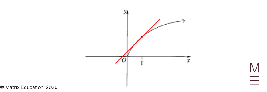
The reply is A. We’ve start{align*} since it’s above the ( x ) -axis. The graph is concave downwards so start{align*} By contemplating the tangent to ( y = f(x) ) that passes via the factors ( (0, c)) and ( (1, f(1))), we now have start{align*} Additionally, the slope of the tangent to ( f(x) ) at ( x = 1 ) is optimistic, so start{align*} In conclusion, start{align*} |
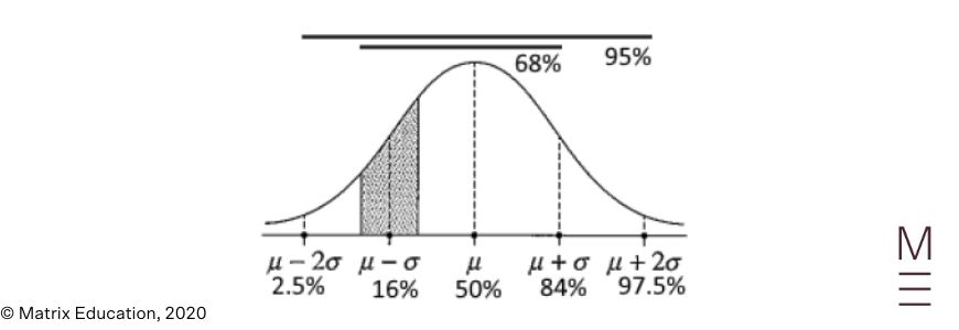
| 9. | C | We will make the next markings on the traditional curves offered:
Solely C then has the decrease sure of ( 10% ) and the higher sure of ( 25% ) within the right areas. |
| 10. | D | There are 2 most stationary factors at (? = 1) and since (?(?)) is steady, there have to be a minimal stationary level in between. Subsequently (3) stationary factors in complete. |
Part 2. Lengthy response
Query 11a
Query 11b
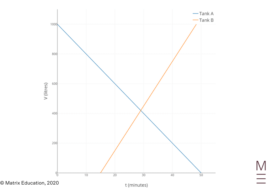
The quantity of water in Tank B is ( V = 30t + b ) . Substituting ( V = 0 ) and ( t = 15 ) into the equation offers
| start{align*} 0 &= 30left(15right) + b 0 &= 450 + b b &= -450 finish{align*} |
Which means that the amount of water in Tank B is
| ( V = 30t – 450) |
It’s provided that the amount of water in Tank A is
| ( V = 1000 – 20t ) |
So the 2 tanks have the identical quantity of water when
| start{align*} 30t – 450 &= 1000 – 20t 1450 &= 50t t &= frac{1450}{50} t &= 29 finish{align*} |
Subsequently, at ( t = 29 ) minutes, they include the identical quantity of water.
Query 11c
When the whole quantity of water within the two tanks is ( 1000 ) litres, we now have
| start{align*} (1000 – 20t) + (30t – 450) &= 1000 550 + 10t &= 1000 t &= frac{1000 – 550}{10} t &= 45 finish{align*} |
Subsequently, at ( t = 45 ) minutes, the whole quantity of water within the two tanks is ( 1000 ) litres.
Query 12
The widespread distinction is
| start{align*} d &= T_2 – T_1 &= 10 – 4 &= 6 finish{align*} |
The primary time period is
| ( a = 4 ) |
Utilizing
| ( T_n = a + (n – 1) d ) |
we now have
| start{equation*} 1354 = 4 + (n – 1) (6) ,, finish{equation*} |
so
| start{align*} n &= frac{1354 – 4}{6} + 1 &= 226 finish{align*} |
Subsequently, the sum of the arithmetic sequence is
| start{align*} S_{226} &= frac{226}{2} (4 + 1354) &= 153454 finish{align*} |
Query 13
We’ve
| start{align*} int_0^{pi/4} sec^2 x , dx &= left[tan xright]_0^{pi/4} &= tan left(frac{pi}{4}proper) – tan left(0right) &= 1 – 0 &= 1 finish{align*} |
Query 14a
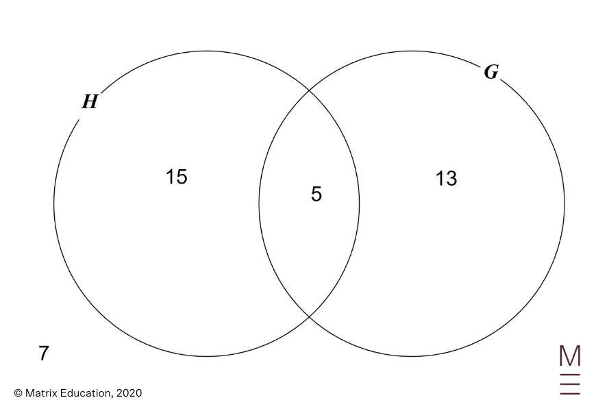
We’ve
| start{align*} n left(H cup Gright) &= n left(Hright) + n left(Gright) – nleft(H cap Gright) 33 &= 20 + 18 – n left(H cap Gright) nleft(H cap Gright) &= 5 ,. finish{align*} |
Subsequently,
| start{align*} Pleft(H cap Gright) &= frac{5}{40} &= frac{1}{8} ,. finish{align*} |
Query 14b
We’ve
| start{align*} P left(overline{H} ,|, Gright) &= frac{Pleft(overline{H} cap Gright)}{Pleft(Gright)} &= frac{13}{18} ,. finish{align*} |
Query 14c
The likelihood required is
| start{align*} Pleft(Hright) instances Pleft(overline{H}proper) &= frac{20}{40} instances frac{20}{39} &= frac{10}{39} ,. finish{align*} |
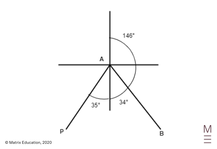
Query 15a
We’ve
| start{align*} angle APB &= angle NPB – angle NPA &= 100º – 35º &= 65º finish{align*} |
as required.
Query 15b
Utilizing the cosine rule, we now have
| start{align*} AB^2 &= AP^2 + PB^2 – 2 instances AP instances PB instances cos 65º &= 7^2 + 9^2 – 2 instances 7 instances 9 instances cos 65º &= 76.75 finish{align*} |
so
| start{align*} AB &= sqrt{76.75} &= 8.76 textual content{km} quad textual content{(right to 2 d.p.)} finish{align*} |
Query 15c
Utilizing the cosine rule, we now have
| start{equation*} PB^2 = AP^2 + AB^2 – 2 instances AP instances AB instances cos (angle PAB) finish{equation*} |
Rearranging this provides
| start{align*} cos (angle PAB) &= frac{AP^2 + AB^2 – PB^2}{2 instances AP instances AB} &= frac{7^2 + 76.75 – 9^2}{2 instances 7 instances 8.76} &= 0.365 finish{align*} |
so
| start{align*} angle PAB &= cos^{-1} left(0.365right) &= 68º 36′ &approx 69º finish{align*} |
Subsequently,
| start{align*} textual content{bearing} &= 180º – (69º – 35º) &= 146º quad textual content{(right to the closest diploma)} ,. finish{align*} |
Query 16
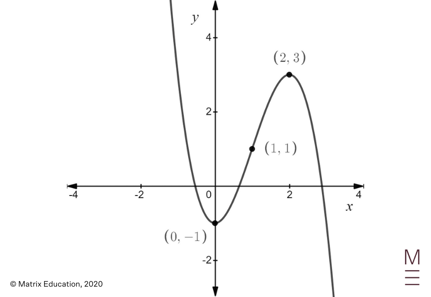
Calculating the derivatives offers
| start{align*} frac{dy}{dx} &= frac{d}{dx} (-x^3 + 3x^2 – 1) &= -3x^2 + 6x &= -3x (x – 2) finish{align*} |
and
| start{align*} frac{d^2 y}{dx^2} & = frac{d}{dx} (-3x^2 + 6x) & = -6x + 6 & = -6(x – 1) finish{align*} |
For the stationary factors, setting ( frac{dy}{dx} = 0 ) offers
| ( -3x (x – 2) = 0 ) |
so
| start{align*} x = 0 quad textual content{or} quad x = 2. finish{align*} |
When ( x = 0 ),
| start{align*} y &= -0^3 + 3 (0)^2 – 1 &= -1 finish{align*} |
When ( x = 2 )
| start{align*} y &= -2^3 + 3(2)^2 – 1 &= 3 finish{align*} |
Subsequently, the stationary factors are ( (0,-1) ) and ( (2, 3) ).
| ( x ) | ( x < 0 ) | ( x = 0 ) | ( 0 < x < 2 ) | ( x = 2 ) | ( x > 2 ) |
| ( frac{dy}{dx} ) | ( – ) | ( 0 ) | ( + ) | ( 0 ) | ( – ) |
For the factors of inflection, setting ( frac{d^2 y}{dx^2} = 0 ) offers
| start{align*} -6(x – 1) = 0 finish{align*} |
So,
| start{align*} x = 1 finish{align*} |
When ( x = 1 ),
| start{align*} y &= -1^3 + 3(1)^2 – 1 &= 1 finish{align*} |
Subsequently, the purpose of inflection is ( (1,1) ).
| ( x ) | ( x < 1 ) | ( x = 0 ) | ( x > 1 ) |
| ( frac{d^{2}y}{dx^{2}} ) | ( + ) | ( 0 ) | ( – ) |
The ( y ) -intercept is
| start{align*} y &= -0^3 + 3(0)^2 – 1 &= -1 finish{align*} |
Query 17
We use integration by substitution. Let ( u = 4 + x^2 ). Then ( frac{du}{dx} = 2x ), so ( du = 2x dx ).
Subsequently,
| start{align*} int frac{x}{4 + x^2} , dx &= int frac{1}{2} left(frac{2x}{4 + x^2}proper) , dx &= int frac{1}{2} left(frac{du}{u}proper) &= frac{1}{2} ln left|uright| + C &= frac{1}{2} ln left|4 + x^2right| + C &= frac{1}{2} ln left(4 + x^2right) + C ,, quad textual content{since $4 + x^2 > 0$} ,, finish{align*} |
The place ( C ) is a continuing.
Query 18a
Utilizing the product rule offers
| start{align*} frac{d}{dx} left(e^{2x} left(2x + 1right)proper) &= e^{2x} frac{d}{dx} left(2x + 1right) + left(2x + 1right) frac{d}{dx} left(e^{2x}proper) &= e^{2x} left(2right) + left(2x + 1right) left(2e^{2x}proper) &= 2e^{2x} + 4xe^{2x} + 2e^{2x} &= 4e^{2x} + 4xe^{2x} &= 4e^{2x} left(1 + xright) ,. finish{align*} |
Query 18b
We’ve
| start{align*} int left(x + 1right) e^{2x} , dx &= frac{1}{4} int 4 left(x + 1right) e^{2x} , dx &= frac{1}{4} left[e^{2x} left(2x + 1right)right] + C ,, finish{align*} |
the place ( C ) is a continuing, utilizing the consequence from half (a).
Query 19
Ranging from the left hand aspect, we now have
| start{align*} sec theta – cos theta &= frac{1}{cos theta} – cos theta &= frac{1 – cos^2 theta}{cos theta} &= frac{sin^2 theta}{cos theta} &= sin theta cdot frac{sin theta}{cos theta} &= sin theta tan theta finish{align*} |
as required.
Query 20
Utilizing the trapezoidal rule, we discover that
| start{align*} textual content{approximate distance} &= frac{frac{1}{60}}{2} left[60 + 2 left(55 + 65 + 68 + 70right) + 67right] &= frac{643}{120} &= 5.358 &=5.4 (1text{ d.p.}) finish{align*} |
Query 21a
The temperate of the tea 4 minutes after it has been poured is discovered by substituting ( t = 4 ) into ( T ) , which supplies
| start{align*} T &= 25 + 70 left(1.5right)^{-0.4 left(4right)} &= 25 + 70 left(1.5right)^{-0.4 left(4right)} &= 25 + 70left(1.5right)^{-1.6} &approx 61.5891 textual content{levels Celsius.} finish{align*} |
Query 21b
The speed of change of the temperature of the tea is
| start{align*} frac{dT}{dt} &= frac{d}{dt} left(25 + 70left(1.5right)^{-0.4t}proper) &= 70left(1.5right)^{-0.4t} left(log_e 1.5right) frac{d}{dt} left(-0.4tright) &= 70left(1.5right)^{-0.4t} left(log_e 1.5right) left(-0.4right) &= left(-28log_e 1.5right) left(1.5right)^{-0.4t} ,. finish{align*} |
When ( t = 4 ) , this turns into
| start{align*} frac{dT}{dt} &= left(-28log_e 1.5right) left(1.5right)^{-0.4 left(4right)} &approx -5.93425 ,, finish{align*} |
which is destructive, so the tea is cooling on the charge of ( 5.93425 ) levels Celsius per minute.
Query 21c
Substituting ( T = 55 ) into ( T = 25 + 70 (1.5)^{-0.4t} ) offers
| start{equation*} 55 = 25 + 70 left(1.5right)^{-0.4t} ,, finish{equation*} |
so
| start{equation*} 30 = 70 left(1.5right)^{-0.4t} ,, finish{equation*} |
and
| start{equation*} frac{3}{7} = left(1.5right)^{-0.4t} ,. finish{equation*} |
Taking logarithms on either side of the equation offers
| start{equation*} log_e left(frac{3}{7}proper) = log_e left(1.5right)^{-0.4t} ,, finish{equation*} |
so
| start{equation*} log_e left(frac{3}{7}proper) = -0.4t log_e left(1.5right) ,, finish{equation*} |
and
| start{align*} t &= -frac{1}{0.4 log_e left(1.5right)} log_e left(frac{3}{7}proper) &approx 5.22423 finish{align*} |
Query 22
Utilizing the given perimeter we now have
| start{align*} AB &= frac{textual content{perimeter}}{textual content{variety of sides}} &= frac{80}{10} &= 8 , textrm{cm} finish{align*} |
We even have
| start{align*} angle AOB &= 360° div 10 &= 36° finish{align*} |
Utilizing the cosine rule offers
| ( AB^2 = AO^2 + BO^2 – 2 instances AO instances BO instances cos angle AOB ) |
Since ( AO = BO ) and ( AB = 8 ), we now have
| start{align*} 8^2 &= AO^2 + AO^2 – 2 instances AO instances AO instances cos 36° 64 &= 2 (AO)^2 – 2 AO^2 cos 36° 64 &= AO^2 (2 – 2 cos 36°) AO^2 &= frac{64}{2 – 2 cos 36°} finish{align*} |
Subsequently,
| start{align*} textual content{space of the decagon} &= 10 instances textual content{space of} triangle textual content{AOB} &= 10 instances left[frac{1}{2} times AO^2 sin 36º right] &= 10 instances frac{1}{2} instances frac{64}{2 – 2 cos 36º} instances sin 36º &= 492.429 &approx 492.4 , textrm{cm}^2 quad textual content{(right to 1 d.p.)} finish{align*} |
Query 23a
Since ( f(x) ) is a likelihood density perform, we all know that
| start{align*} int_0^ok sin x , dx &= 1 left[-cos xright]_0^ok &= 1 – cos ok – left(- cos 0right) &= 1 – cos ok + 1 &= 1 cos ok &= 0 , finish{align*} |
Fixing this for ( ok ) offers
| ( ok = frac{pi}{2} ) |
Query 23b
Since ( 1 < frac{pi}{2} ), we now have
| start{align*} Pleft(X leq 1right) &= int_0^1 fleft(xright) , dx &= int_0^1 sin x , dx &= left[-cos xright]_0^1 &= -cos 1 – left(- cos 0right) &= – cos 1 + 1 &= 0.4597 ,. finish{align*} |
Query 24
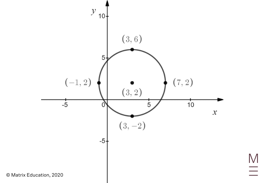
Beginning with the circle given, we full the sq. and acquire
| start{align*} x^2 – 6x + y^2 + 4y – 3 &= 0 x^2 – 6x + y^2 + 4y &= 3 left(x^2 – 6x + 9right) + left(y^2 + 4y + 4right) &= 3 + 9 + 4 left(x – 3right)^2 + left(y + 2right)^2 &= 16 finish{align*} |
Which means that the unique circle is centred at ( (3, -2) ) and its radius is ( 4 ) models.
When it’s mirrored within the ( x ) -axis, we multiply the ( y ) -coordinate by ( -1 ) so the centre of the mirrored circle is ( (3,2) ) , and the radius remains to be ( 4 ) models.
Query 25a
The radius of the quarter circle is ( x ) metres. We’ve
| start{align*} textual content{space of backyard mattress} &= textual content{space of rectangle} + textual content{space of quarter circle} &= xy + frac{1}{4} left(pi x^2right) ,. finish{align*} |
Since this must be equal to ( 36 ), we now have
| start{align*} xy + frac{1}{4} left(pi x^2right) &= 36 xy &= 36 – tfrac{1}{4} left(pi x^2right) y &= frac{36}{x} – frac{pi x}{4} ,. finish{align*} |
Subsequently, the perimeter is given by
| start{align*} P &= x + y + left(x + yright) + frac{1}{4} left(2 pi xright) &= 2 left(x + yright) + frac{pi x}{2} &= 2 left[x + left(frac{36}{x} – frac{pi x}{4}right)right] + frac{pi x}{2} &= 2x + frac{72}{x} – frac{pi x}{2} + frac{pi x}{2} &= 2x + frac{72}{x} ,, finish{align*} |
as required.
Query 25b
First, we differentiate ( P = 2x + frac{72}{x}) and acquire
| start{align*} frac{dP}{dx} &= frac{d}{dx} left(2x + frac{72}{x}proper) &= 2 – frac{72}{x^2} ,. finish{align*} |
Setting ( frac{dP}{dx} = 0 ) offers ( 2 – frac{72}{x^2} = 0 ). Which means that
| ( frac{72}{x^2} = 2 ) |
so
| ( x^2 = 36 ) |
and
| ( x = 6 ) |
since ( x ) is the dimension of a rectangle and it have to be non-negative. When ( x = 6 ), the perimeter is given by
| start{align*} P &= 2 left(6right) + frac{72}{6} &= 12 + 12 &= 24 textual content{metres} finish{align*} |
| ( x ) | ( 0 < x < 6 ) | ( x = 6 ) | ( x > 6 ) |
| ( frac{dP}{dx} ) | ( – ) | ( 0 ) | ( + ) |
Subsequently, ( P = 24 ) is the smallest doable perimeter.
Query 26a
We use the recurrence relation beginning with
| ( A_0 = 60000 ) |
The sum of money within the account after the primary withdrawal is
| start{align*} A_1 &= A_0 left(1.005right) – 800 &= 60000 left(1.005right) – 800 ,, finish{align*} |
The sum of money within the account after the second withdrawal is
| start{align*} A_2 &= A_1 left(1.005right) – 800 &= left[60000 left(1.005right) – 800right] left(1.005right) – 800 &= 60000 left(1.005right)^2 – 800 left(1 + 1.005right) ,, finish{align*} |
And the sum of money within the account after the third withdrawal is
| start{align*} A_3 &= A_2 left(1.005right) – 800 &= left[60000 left(1.005right)^2 – 800 left(1 + 1.005right)right] left(1.005right) – 800 &= 60000 left(1.005right)^3 – 800 left(1 + 1.005 + 1.005^2right) &approx 58492.49 quad textual content{(right to 2 d.p.)} ,. finish{align*} |
Query 26b
The curiosity within the first month is
| start{align*} I_1 &= A_0 instances 0.5% &= 60000 instances 0.005 &= $ 300 finish{align*} |
The curiosity within the second month is
| start{align*} I_2 &= A_1 instances 0.5% &= left(60000 instances 1.005 – 800right) instances 0.005 &= $ 297.50 finish{align*} |
The curiosity within the third month is
| start{align*} I_3 &= A_2 instances 0.5% &= left(60000 instances 1.005^2 – 800 instances 1.005 – 800right) instances 0.005 &= $ 294.99 finish{align*} |
Subsequently, the whole quantity of curiosity earned within the first three months is
| start{align*} I_1 + I_2 + I_3 &= $ 892.49 finish{align*} |
Query 26c
The sum of money within the account instantly after the 94th withdrawal is
| start{align*} A_{94} &= A_{93} left(1.005right) – 800 &= 60000 instances 1.005^{94} – 800 instances left(1 + 1.005 + 1.005^2 + dots + 1.005^{93}proper) &= 60000 instances 1.005^{94} – 800 instances left(frac{1 – 1.005^{94}}{1 – 1.005}proper) &= $ 187.85 quad textual content{right to 2 decimal locations} finish{align*} |
Query 27
From the field plot, the median of the temperature is ( 22 ) levels Celsius. It’s provided that the imply temperature is ( 0.525 ) levels beneath the median temperature, so
| start{align*} bar{x} &= 22 – 0.525 &= 21.475 textual content{levels Celsius} finish{align*} |
The common variety of chirps over the 20 days is
| start{align*} bar{y} &= frac{684}{20} &= 34.2 finish{align*} |
Taking the anticipated worth of either side of
| (y = -10.6063 + bx ) |
offers
| (bar{y} = -10.6063 + b bar{x} ) |
so
| ( 34.2 = -10.6063 + b left(21.475right) ) |
and
| start{align*} b &= frac{34.2 + 10.6063}{21.475} &= 2.08644004657 finish{align*} |
Which means that
| ( y = -10.6063 + 2.08644004657x ) |
Subsequently, the variety of chirps anticipated in a 15-second interval when the temperature is nineteen levels Celsius is discovered by substituting ( x = 19 ), giving
| start{align*} y &= -10.6063 + 2.08644004657 left(19right) &approx 29 quad textual content{(right to the closest complete quantity)} ,. finish{align*} |
Query 28a
Let ( X ) {dollars} be the hourly charge of pay for adults who work. We’re provided that ( X sim mathcal{N} left(25, 5^2right) ) , so the likelihood that an grownup earns between ( $ 15 ) and ( $30 ) per hour is
| start{align*} Pleft(15 leq X leq 30right) &= Pleft(frac{15 – 25}{5} leq frac{X – 25}{5} leq frac{30 – 25}{5}proper) &= Pleft(-2 leq Z leq 1right) &= 0.84134 – 0.02275 &= 0.81859 finish{align*} |
Subsequently,
| start{align*} Pleft(textual content{an grownup’s hourly charge of pay will not be between $15 and $30}proper) &= 1 – Pleft(15 leq X leq 30right) &= 1 – 0.81859 &= 0.18141 finish{align*} |
and
| start{align*} Pleft(textual content{not less than one in all two adults earns between $15 and $30}proper) &= 1 – Pleft(textual content{neither earns between $15 and $30 an hour}proper) &= 1 – 0.18141^2 &= 0.9671 finish{align*} |
Query 28b
For the reason that variety of adults who work is the same as thrice the variety of adults who don’t work, we all know that
| start{equation*} P left(textual content{a randomly chosen grownup works}proper) = frac{1}{4} finish{equation*} |
Which means that
| start{align*} &∴P left( textual content{Chosen grownup works and earns greater than} $25 textual content{ per hour} proper) = frac{3}{4} instances frac{1}{2} & =frac{3}{8} finish{align*} |
Query 29a
Since
| start{align*} frac{dy}{dx} &= frac{d}{dx} left(c ln xright) &= frac{c}{x} ,, finish{align*} |
the slope of the tangent to ( y = c ln x ) at ( x = p ) is
| (frac{dy}{dx}bigg|_{x = p} = frac{c}{p} ) |
When ( x = p ), the corresponding ( y )-coordinate is
| start{equation*} y = c ln p finish{equation*} |
Which means that the equation of the tangent to ( y = c ln x ) at ( x = p ) is given by
| start{equation*} frac{y – c ln p}{x – p} = frac{c}{p} finish{equation*} |
Multiplying either side by ( x – p ) offers ( y – c ln p = frac{c}{p} left(x – pright) ), so
| start{align*} y &= frac{c}{p} left(x – pright) + c ln p &= frac{c}{p} x – c + c ln p ,, finish{align*} |
as required.
Query 29b
For the reason that tangent has a gradient of ( 1 ), we now have
| start{equation} label{eq:Q29bEq1} frac{c}{p} = 1 finish{equation} |
which signifies that
| start{equation} label{eq:Q29bEq2} c = p finish{equation} |
Moreover, because the tangent passes via the origin, substituting ( x = 0 ) and ( y = 0 ) into the equation of the tangent offers
| start{equation*} 0 = frac{c}{p} left(0right) – c + c ln p finish{equation*} |
which signifies that ( 0 = -c + c ln p ), or equivalently,
| start{equation} label{eq:Q29bEq3} c left(-1 + ln pright) = 0 finish{equation} |
From Eq. ( frac{c}{p} = 1), we all know that ( c neq 0 ), so Eq. ( c left(-1 + ln pright) = 0 ) implies that
| start{equation*} -1 + ln p = 0 ,, finish{equation*} |
which signifies that
| start{equation*} ln p = 1 ,, finish{equation*} |
and
| start{equation} label{eq:Q29bEq4} p = e finish{equation} |
Substituting ( p = e ) into ( c = p ) offers
| start{equation*} c = e ,. finish{equation*} |
Query 30a
Since ( A ) is the purpose of intersection of
| start{equation*} y = 4x – x^2 finish{equation*} |
and
| start{equation*} y = ax^2 finish{equation*} |
its ( x ) -coordinate is discovered by equating each equations and fixing for ( x ). This offers
| start{equation*} 4x – x^2 = ax^2 finish{equation*} |
so
| start{equation*} left(1 + aright) x^2 – 4x = 0 finish{equation*} |
or equivalently,
| start{equation*} x left [ left(1 + a right )x – 4 right] = 0 finish{equation*} |
Both ( x = 0 ) or ( left(1 + aright) x – 4 = 0 ), however from the diagram we see that the ( x ) coordinate of ( A ) will not be ( 0 ), which signifies that we will need to have
| start{equation*} left(1 + aright) x – 4 = 0 finish{equation*} |
Rearranging this provides
| start{equation*} left(1 + aright) x = 4 finish{equation*} |
so
| start{equation*} x = frac{4}{1 + a} finish{equation*} |
as required.
Query 30b
The shaded space is given by
| start{align*} int_0^{4/left(1+aright)} left[left(4x – x^2right) – ax^2right] , dx &= int_0^{4/left(1+aright)} left[left(4x – x^2right) – ax^2right] , dx &= int_0^{4/left(1+aright)} left(4x – x^2 – ax^2right) , dx &= left[2x^2 – frac{x^3}{3} – frac{ax^3}{3}right]_0^{4/left(1+aright)} &= 2left(frac{4}{1 + a}proper)^2 – frac{1}{3} left(frac{4}{1 + a}proper)^3 – frac{a}{3} left(frac{4}{1 + a}proper)^3 &= frac{32}{left(1 + aright)^2} – frac{64}{3 left(1 + aright)^3} – frac{64a}{3left(1 + aright)^3} &= frac{96 left(1 + aright) – 64 -64a}{3left(1 + aright)^3} &= frac{96 + 96a – 64 -64a}{3left(1 + aright)^3} &= frac{32 left(1 + aright)}{3left(1 + aright)^3} &= frac{32}{3left(1 + aright)^2} finish{align*} |
Subsequently, to ensure that the shaded space to be equal to ( frac{16}{3} ), we want
| start{equation*} frac{32}{3left(1 + aright)^2} = frac{16}{3} finish{equation*} |
which implies
| start{equation*} left(1 + aright)^2 = 2 finish{equation*} |
Subsequently,
| start{equation*} 1 + a = pm sqrt{2} finish{equation*} |
so ( a = -1 pm sqrt{2} ). From the diagram, we want ( a > 0 ), so
| start{equation*} a = -1 + sqrt{2} finish{equation*} |
Query 31a
( a ) represents the amplitude, so
| start{align*} a &= frac{35000 – 5000}{2} &= 15000 finish{align*} |
( b ) represents the vertical displacement, so
| start{align*} b &= 35000 – 15000 &= 20000 finish{align*} |
Query 31b
Differentiating ( mleft(tright) ) offers
| start{equation*} m’left(tright) = 15000left(frac{pi}{26}proper) cos left(frac{pi}{26} tright) finish{equation*} |
For ( mleft(tright) ) to be growing, we assess when ( m’left(tright) > 0 ). This happens when
| start{equation*} cos left(frac{pi}{26} tright) > 0 finish{equation*} |
So
| start{equation*} frac{pi}{26} t < frac{pi}{2} quad textual content{or} quad frac{pi}{26} t > frac{3 pi}{2} finish{equation*} |
Which means that
| start{equation*} t < 13 quad textual content{or} quad t > 39 finish{equation*} |
Likewise with ( cleft(tright) ), and we now have
| start{equation*} c’left(tright) = frac{80 pi}{26} sin left[frac{pi}{26} left(t – 10right)right] finish{equation*} |
Now, ( c’left(tright) > 0 ) happens when
| start{equation*} sin left[frac{pi}{26} left(t – 10right)right] > 0 finish{equation*} |
which signifies that
| start{equation*} 0 < frac{pi}{26} left(t – 10right) < pi finish{equation*} |
so
| start{equation*} 10 < t < 36 finish{equation*} |
Subsequently, each populations are growing when
| start{equation*} 10 < t < 13 finish{equation*} |
Query 31c
First, we discover when ( cleft(tright) ) reaches a most. This happens when ( c’left(tright) = 0 ), so
| start{equation*} frac{80 pi}{26} sin left[frac{pi}{26} left(t – 10right)right] = 0 ,, finish{equation*} |
or equivalently,
| start{equation*} sin left[frac{pi}{26} left(t – 10right)right] = 0 ,. finish{equation*} |
Subsequently,
| start{equation*} frac{pi}{26} left(t – 10right) = 0 quad textual content{or} quad frac{pi}{26} left(t – 10right) = pi ,, finish{equation*} |
and the stationary factors are
| start{equation*} t = 10 quad textual content{or} quad t = 36 ,. finish{equation*} |
To find out the character of those stationary factors, we look at ( c”left(tright) ). Now,
| start{equation*} c”left(tright) = frac{80 pi^2}{26^2} cos left(frac{pi}{26} left(t – 10right)proper) ,. finish{equation*} |
At ( t = 36 ),
| start{align*} c”left(36right) &= -1.168 &< 0 finish{align*} |
so ( cleft(tright) ) attains its most when ( t = 36 ). At (t = 36 ) ,
| start{align*} m’left(36right) &= frac{15000pi}{26} cos left(frac{36 pi}{26}proper) &= -642.7 finish{align*} |